INDEL

The INDEL family classifies contiguous coding mismatches into a structural error taxonomy instead of reducing them to a single overlap score. Each mismatch run is additionally typed by the semantic position of the GT exon it touches — five_prime_terminal_exon, internal_exon, three_prime_terminal_exon, or single_exon_gene — so a slip on a 5′-terminal exon is kept separate from one on an internal exon even though both look identical to the binary coding mask.

Example Plots

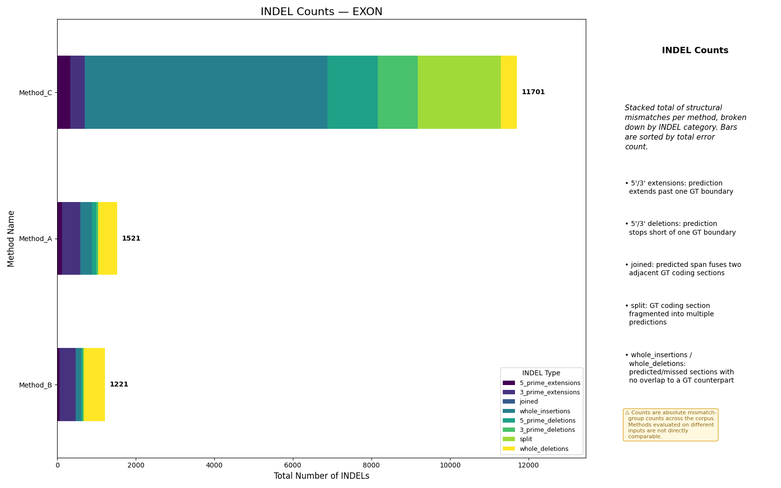
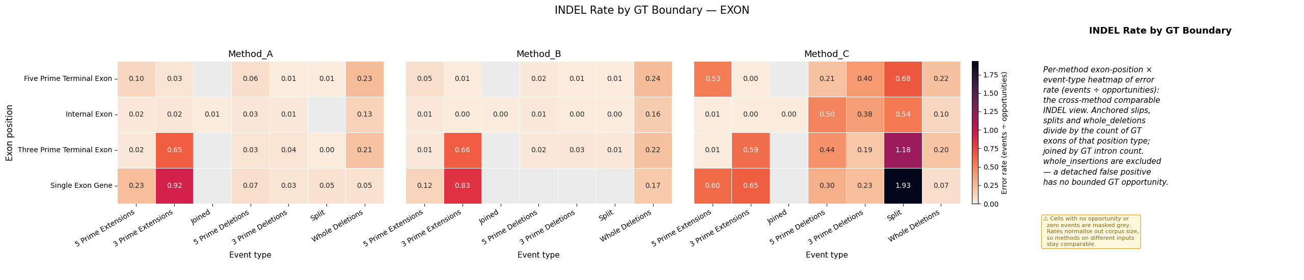
Four complementary views are produced (all boundary-resolved views use one panel per method over a shared, biologically-ordered grid, so methods compare directly):

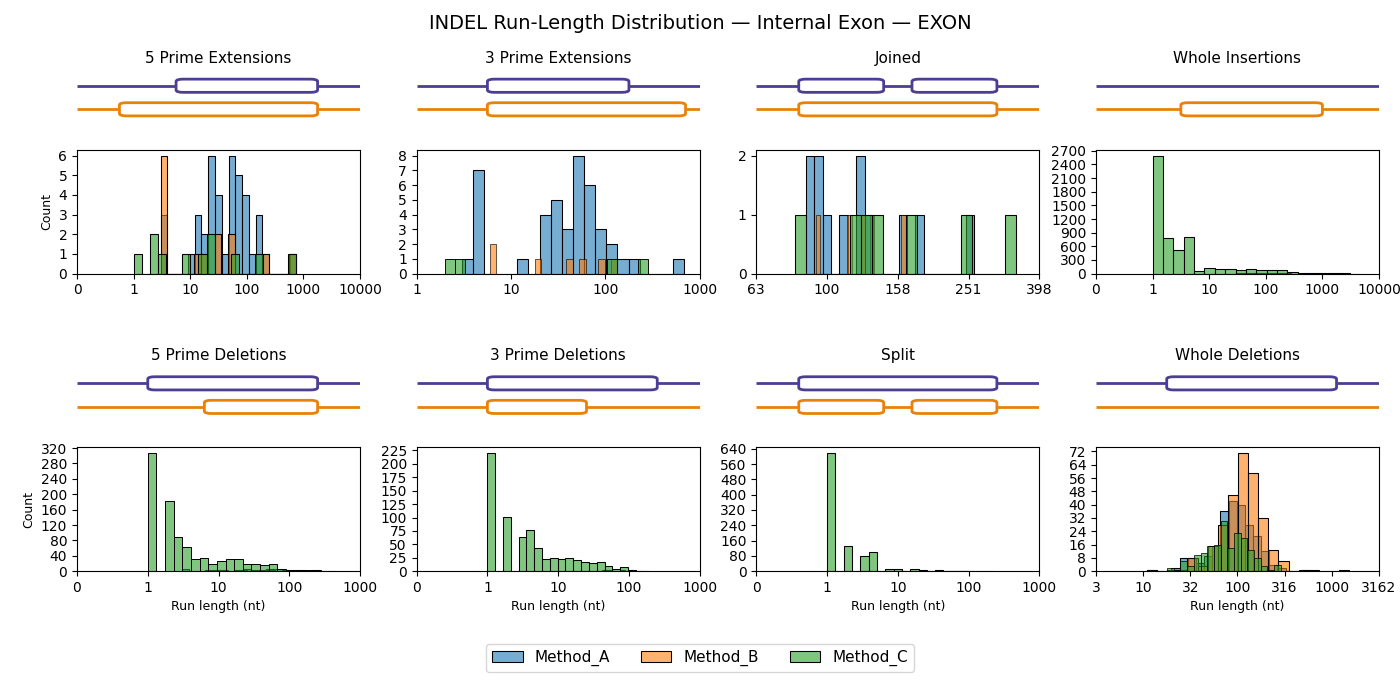
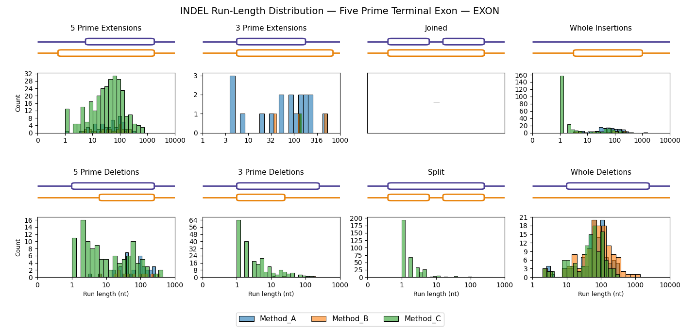
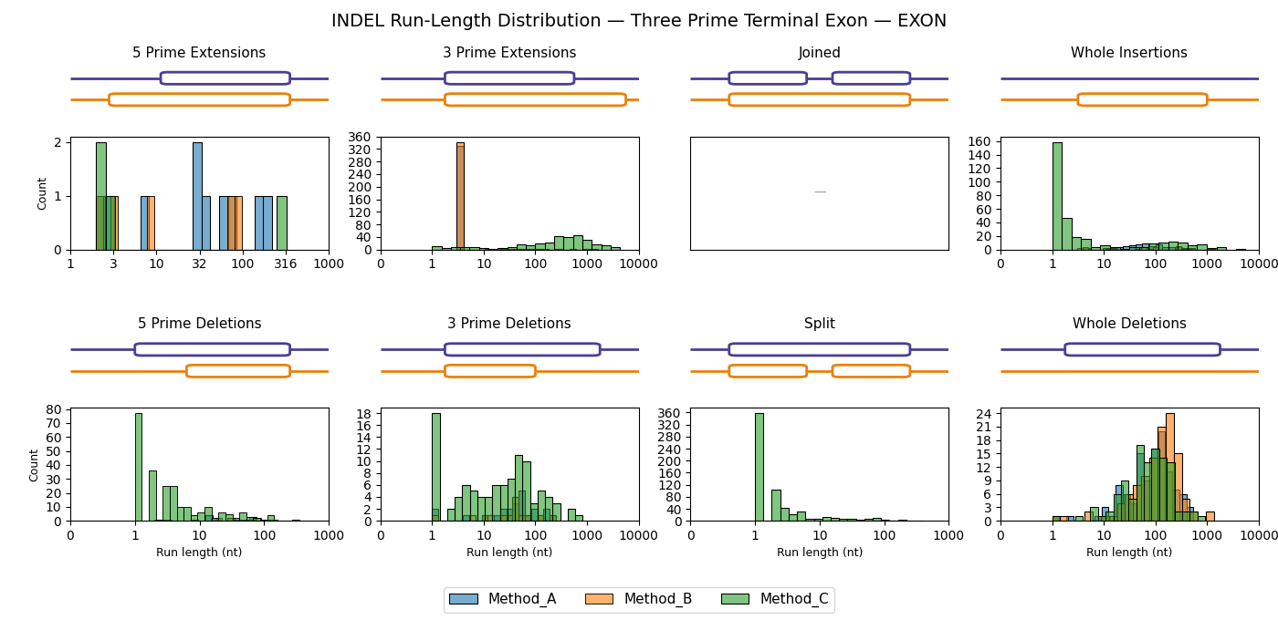
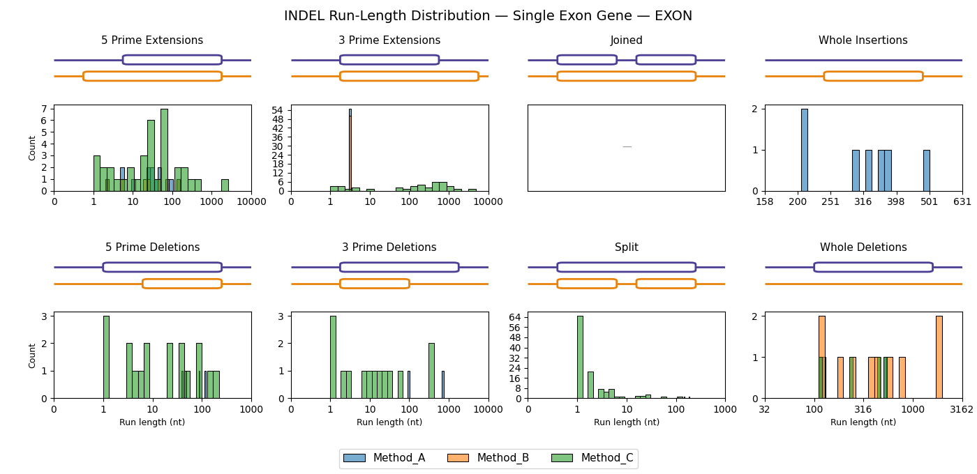
• indel_counts — per method, the total number of each structural error type (boundaries aggregated). Answers which error types dominate.

• indel_rates_by_boundary — the headline benchmarking view: a GT-boundary × event-type rate heatmap (events ÷ opportunities; see Rates below). Colour = rate, cell annotation = raw count, grey = no opportunity. Answers how reliably each method handles each junction, comparably across methods and junction types.

• indel_counts_by_boundary — the raw-magnitude companion: the same grid coloured by event count on a log scale (so one huge cell does not wash out the rest). Answers where the errors concentrate in absolute terms.

• indel_lengths_<boundary> — one figure per exon-position category: a 4 × 2 grid (insertions top row, deletions bottom row) of overlaid per-method run-length histograms. Answers how large the slips are at each junction, separating small boundary slips from long insertions/deletions or broad merge/split regions.

Run-length distributions by exon position

Internal exon

5′ terminal exon

3′ terminal exon

Single-exon gene

Categories

Insertions are runs where the prediction has coding and GT does not:

• 5_prime_extensions

• 3_prime_extensions

• joined

• whole_insertions

Deletions are runs where GT has coding and the prediction does not:

• 5_prime_deletions

• 3_prime_deletions

• split

• whole_deletions

How Classification Works

The benchmark pads the GT and prediction coding masks with one background position on both sides. For each contiguous mismatch run it checks whether the run touches a correct coding region (coding in both GT and prediction) immediately on the 5’ side, the 3’ side, both, or neither.

That local neighborhood test drives the event type:

• one touched side: extension or deletion at that end

• both touched sides: joined or split

• neither side: whole insertion or whole deletion

Exon-Position Typing

On top of the event type, each run is keyed by the semantic position of the GT exon it touches, one of four categories:

• five_prime_terminal_exon

• internal_exon

• three_prime_terminal_exon

• single_exon_gene

Each GT coding segment is typed once from the GT labels immediately flanking it (semantic_boundary_label): a flank is terminal when it is outside the intron chain (NONCODING, the sequence edge none, or a UTR label marking the start/stop-codon boundary in UTR_CDS_INTRON mode); INTRON is the only internal flank. Two terminal flanks → single_exon_gene; one terminal flank → 5′- or 3′-terminal exon; two intron flanks → internal_exon.

The run is then keyed by the GT exon it affects, not just its immediate flank:

• deletions are GT-coding throughout, so they key to the exon they sit on;

• 5′/3′ extensions key to the adjacent GT exon they extend;

• joins bridge two exons across an intron → always internal_exon;

• whole insertions have no GT exon under them, so they key to the predicted exon they sit on (typed the same way from the prediction’s flanks).

Because typing reads the flanks in array (5’→3’) order, the 5′- and 3′-terminal categories stay distinct — a distinction a class-blind metric cannot make, since UTR/non-coding appears at both ends of a gene. This is only biologically meaningful under the standard 5’→3’ input orientation (see Conventions).

Output Structure

eval_indel returns

{
    "by_boundary": {exon_type: {event_type: [run_length, ...]}},
    "exon_opportunities": {exon_type: int},  # GT exon count per position type
    "n_gt_segments": int,                    # GT coding segments
    "n_pred_segments": int,                  # predicted coding segments
}

exon_type is one of the four SEMANTIC_BOUNDARY_ORDER categories above. Only run lengths (in nucleotides) are stored, not index arrays: that is all the plots need, and it keeps the per-exon-type fan-out small. The semantic-type keys are produced once, where label_config is available, so the same string keys are used by the tests, the accumulator merge, the plots, and JSON output. The denominators are summed across sequences by the accumulator.

Rates and opportunities

Raw counts are not comparable across methods, test sets, or junction types because they have no denominator. Each event is therefore divided by its opportunity count to give a rate, with a denominator chosen per event family:

event family	events	denominator (opportunity)	reads as
exon-anchored	5’/3’ extensions & deletions, split, whole_deletions	count of GT exons of that position type (exon_opportunities[type])	fraction of that exon type that suffered the error
intron-anchored	joined	GT intron count (n_gt_segments − n_genes)	fraction of introns bridged
gene / intron	whole_insertions	gene count at a terminal exon, intron count internally; unbounded at single_exon_gene (masked)	fraction of that opportunity hallucinated

n_genes = #five_prime_terminal_exon + #single_exon_gene; the plotter derives gene and intron counts from exon_opportunities + n_gt_segments, which assumes each evaluation window is one complete transcript (true under per-transcript scoping).

This split is deliberate: exon-anchored slips measure localization of an exon the method got roughly right, whereas whole_* events are detection (presence/absence) — closer to recall (whole_deletions) and precision (whole_insertions). The indel_rates_by_boundary plot colours by these rates; cells with zero opportunity are masked.

Interpretation

• many 3_prime_extensions / 3_prime_deletions: systematic end-boundary problems

• many joined: the model tends to merge adjacent GT coding sections

• many split: the model fragments single GT coding sections

• many whole_insertions: strong hallucination behavior

• a hotspot at one exon position in indel_counts_by_boundary (e.g. internal_exon 3’-deletions): the model consistently fails one specific exon type. Read it together with the state-transition direction (late vs premature) for the same boundary — INDEL gives the slip magnitude, transitions give the timing.

Caveats

• This taxonomy is scope-specific. “Insertion” / “deletion” are defined relative to the configured evaluation_scope positive-token set (see Annotation Modes). The event type comes from the binary coding mask; the boundary type then restores the GT label context (intron vs UTR vs background) that the mask discards.

• The exon-position key describes which GT (or, for whole insertions, predicted) exon a run touches, not its interior. A run whose interior spans several GT labels (e.g. a hallucinated coding stretch over UTR–intron–UTR) is typed by the single exon it anchors to, collapsing the internal structure.

• It is local. It classifies contiguous mismatch runs, not full transcript structure.

• 5’/3’ and the boundary key order refer to array orientation, not biological strand. Minus-strand input in genomic coordinates would invert the labels. See Conventions.

• The run-length distribution plots use a log10 x-axis with tick labels re-projected to linear bp. A peak labelled “100” represents bins near 100 bp, not exactly 100.