Transition Analysis

Transition analysis answers a different question from the metric families: what happens exactly at label changes, and where does the model introduce spurious changes when GT stays stable?

Requested via EvalMetrics.STATE_TRANSITIONS (kept in the default metric set, so it runs unless an explicit metrics list omits it). When enabled, the outputs appear in aggregated benchmark results as:

• transition_failures

• false_transitions

Transition analysis honours evaluation_scope: out-of-scope exonic content is demoted to background before the arrays are compared, so under the cds scope 5’/3’ UTR read as NONCODING and a UTR-aware prediction is not penalised against a CDS-only ground truth. INTRON and splice labels are always kept, and the default transcript_exon scope demotes nothing.

GT Transition Confusion Matrices

At every position where the GT label changes, the benchmark records:

• the GT source label

• the GT target label

• the predicted target label at the same transition, but only for exact on-site transitions where the prediction is still in the GT source state immediately before the boundary

The result is one confusion matrix per GT source label.

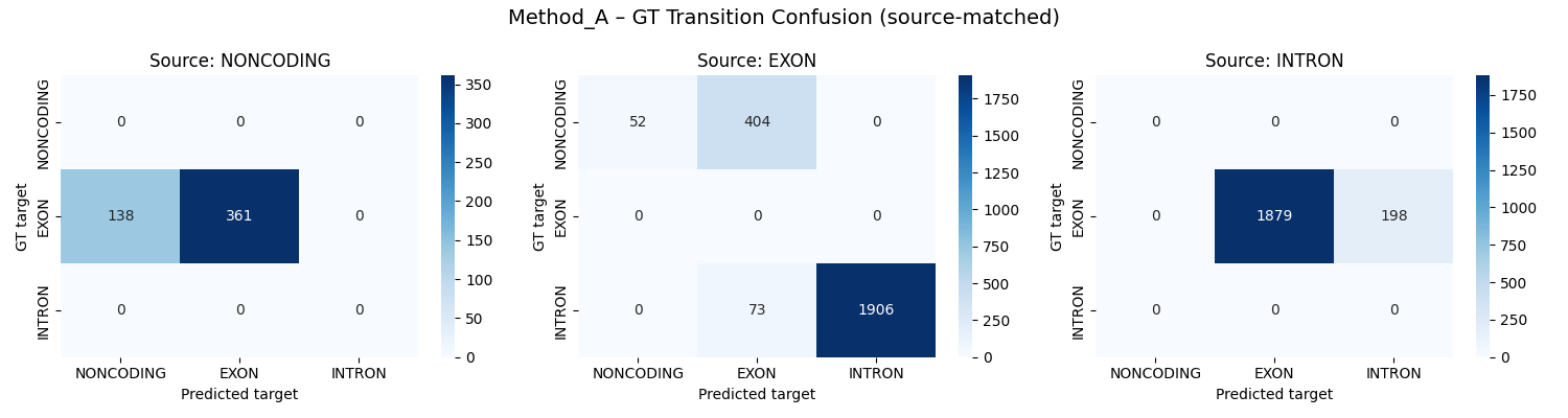
How to read it:

• rows: GT target label

• columns: predicted target label

• one panel: one GT source label

Interpretation:

• mass on the diagonal: the model usually transitions into the correct target label

• mass off the diagonal: the model sees a transition but assigns the wrong target class

• boundaries that were reached too early, too late, or from the wrong source state are intentionally left out here and are instead represented in the false-transition analysis below

This is useful when a model roughly detects exon boundaries but confuses exon, intron, donor, or acceptor labels around those boundaries.

False Transitions

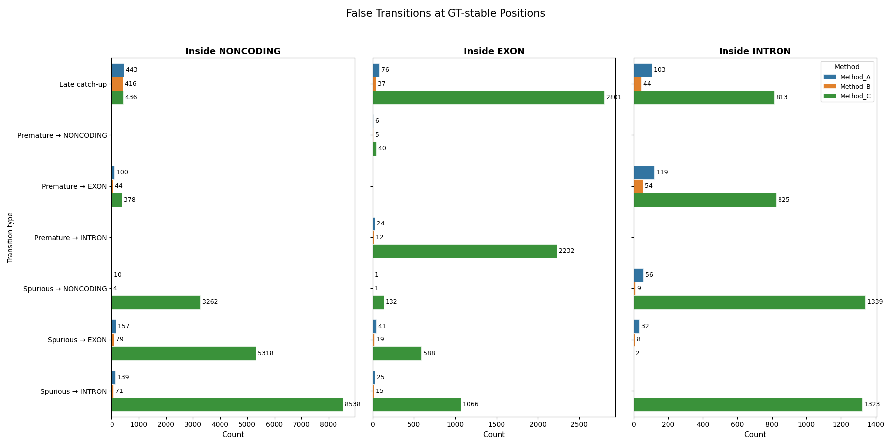
False transitions are counted at positions where GT stays on the same label but the prediction changes label, plus off-track predictions caught at a GT boundary (the prediction had already left the GT source state when GT itself changes — see Caveats).

Each false transition is classified against the GT-stable run it falls in (current label L, preceding label P, following label N) — the predictor’s whole trajectory across that run decides, not the labels of the single transition:

• Late catch-up: the model entered the run still in P and its first transition inside the run is P -> L. It stayed in the previous GT label too long and only now catches up.

• Premature -> X: the model leaves the run in N and its last transition inside the run is L -> N. It left the GT label early and stayed out.

• Spurious -> X: every other transition inside the run — a fabrication the local GT trajectory cannot explain (an invented intron carved out of a real exon, an exon invented inside a real intron, a gene hallucinated in intergenic space).

The anchors are what make a slip a slip: a genuine early exit stays exited. A round-trip excursion (leave the state and come back within the same GT-stable run) is a fabrication and counts as spurious on both of its transitions — so late_catchup / premature measure displaced boundaries, and spurious measures invented ones.

There can be spurious transitions to the same label, e.g. NONCODING -> NONCODING since another spurious transition before transitioned out of NONCODING. Late catch-up and premature transitions exclusively happen at the edges of a coding region if the predicted up or downstream label is continous and does not change up to the GT transition.

Interpretation:

• many false transitions inside EXON: fragmentation of coding segments

• many false transitions inside INTRON: unstable intron labeling or noisy splice handling

• strong Late catch-up: boundaries are found, but shifted downstream

When To Look At These Plots

These plots are especially useful when:

• Region Discovery looks acceptable, but transcript structure is still weak

• one model seems over-fragmented

• splice-site labels are present and you want to see exactly which transitions are confused

Caveats

• Transition analysis is local. It complements transcript-level metrics rather than replacing them.

• Large transition counts do not always imply large biological errors; a model can make many local label mistakes within one otherwise recognizable transcript.

• The false-transition plot shows raw counts, not rates. The benchmark also emits stable_position_counts (positions per label where GT was stable), which is the natural denominator for rates, but the plotting layer does not divide by it. This means a method evaluated on a longer corpus, or on a label that simply occurs more often, will look worse even if its per-position error rate is identical. Compare counts only across runs that share the same input set, or normalise by stable_position_counts yourself when comparing methods on different inputs. Note stable_position_counts counts only GT-stable positions, so it slightly undercounts the true denominator for spurious (which also absorbs off-track events landing at transitioning GT positions) — treat the resulting rate as an upper bound.

• The per-source-label confusion matrices count only on-site transitions where the prediction was already in the GT source state. Off-track predictions (model already left the GT source state when GT changes) are pushed into the spurious bucket, not the GT confusion matrix.

• At array edges (no earlier or later GT transition exists), the lookbehind / lookahead values default to the current GT label as a sentinel that can never match — so edge positions are never classified as late_catchup or premature.

• plot_false_transitions returns None (no figure) when no method has any false transitions, so the figure key is silently absent rather than appearing as an empty plot.