Structural Coherence

Structural Coherence evaluates transcript structure as a whole rather than one coding section at a time. It focuses on whether a predicted set of coding segments (exons/CDS) and the implicit intron boundaries form the same transcript-level structure as the ground truth.

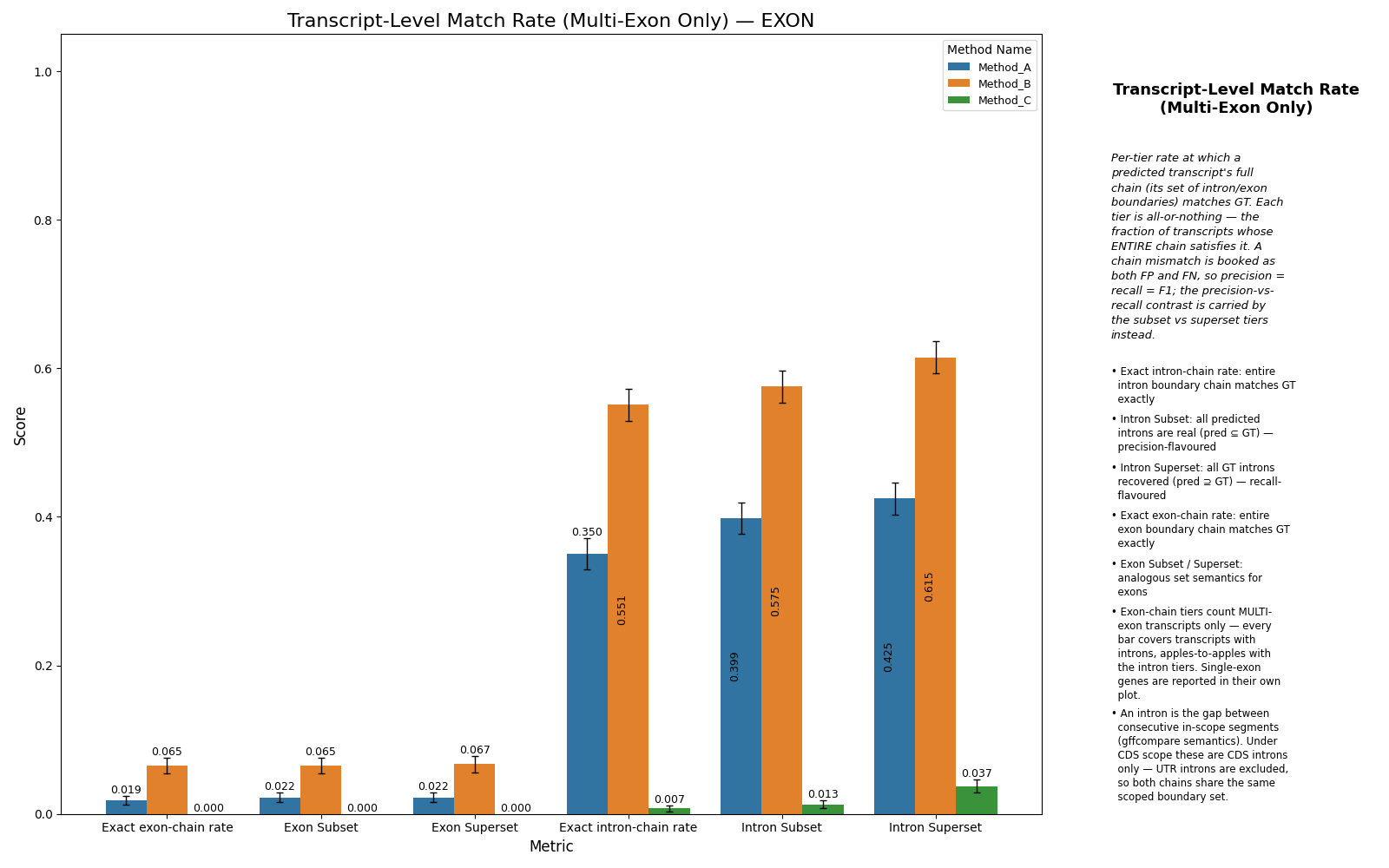
Intron/Exon Chain Match Rate (Multi-Exon Only)

Chain metrics measure whether the complete set of intron or exon boundaries in a predicted transcript matches the ground truth. For each chain type the benchmark reports three sibling metrics:

{chain} — strict exact-match: true only when the predicted boundary set equals the GT boundary set exactly (e.g. intron_chain, exon_chain).
{chain}_subset — true when the predicted set is a subset of GT (every predicted boundary exists in GT). This is precision-oriented: it penalises hallucinated boundaries.
{chain}_superset — true when the predicted set is a superset of GT (every GT boundary is recovered). This is recall-oriented: it penalises missed boundaries.

Population scope: the exon-chain tiers come in two populations. The bare exon_chain / exon_chain_subset / exon_chain_superset keys cover all GT transcripts (single- and multi-exon alike) and are the directly gffcompare-comparable headline (“fraction of transcripts fully recovered”). The exon_chain_multi* variants restrict the same comparison to multi-exon transcripts only, keeping them apples-to-apples with the intron-chain tiers (which are inherently multi-exon). Single-exon genes are also reported separately — see Single-Exon Match Rate below.

For a single (GT, prediction) pair the strict metric is all-or-nothing:

tp = 1 only if the GT set equals the prediction set exactly
otherwise fp = 1 and fn = 1

Aggregation converts those raw counts into corpus-level precision and recall (micro-averaged: counts are summed across sequences before the ratio is taken).

Why a single rate (precision = recall = F1)

Because a chain mismatch is booked as both a false positive and a false negative, every transcript contributes either tp=1 (exact match) or fp=1, fn=1 (anything else). Summed across the corpus this forces FP == FN exactly, so:

precision = TP / (TP + FP) and recall = TP / (TP + FN) come out identical, and
the bootstrap resamples FP and FN with the same indices, so even their standard errors coincide.

Precision and recall therefore carry no independent information for these all-or-nothing tiers — they are the same number (and equal to F1). Reporting them as two separate plots produced the same figure twice, so the benchmark collapses them into a single per-tier match rate. The precision-vs-recall question you actually care about is answered by the tiers themselves: {chain}_subset is the precision-flavoured view (penalises false boundaries) and {chain}_superset is the recall-flavoured view (penalises missed boundaries).

Empty-prediction handling

The subset and superset variants treat the empty prediction case explicitly: an empty prediction is not vacuously a subset of GT. The check requires the predicted set to be non-empty and satisfy the set relation. So a transcript with no predicted segments scores {tp: 0, fp: 1, fn: 1} in every chain variant.

If the GT set itself is empty (no segments of this class for the sequence), the chain comparison contributes nothing — {tp: 0, fp: 0, fn: 0} — so transcripts without coding segments do not artificially inflate or deflate the corpus precision/recall.

Important: introns are always derived positionally from the gaps between consecutive in-scope segments (gffcompare-style) — the scoring never checks whether those gap positions carry an explicit intron label, so introns are inferred from coding-segment gaps regardless of intron labeling. The only error case is a config-level one: if label_config.intron_label is unset in the LabelConfig, intron-chain scoring raises. That is a one-time precondition on the config, not a per-structure content check.

Intron/exon chain match rate (multi-exon only)

Single-Exon Gene Match Rate

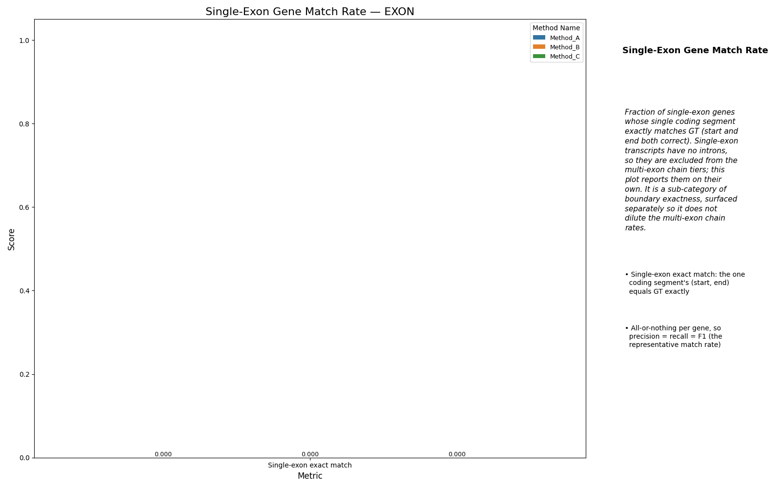
Single-exon transcripts have no introns, so they are excluded from all chain-tier plots above. The single-exon match rate reports how often the one coding segment’s (start, end) matches GT exactly — an all-or-nothing boundary check surfaced in its own plot so it does not dilute the multi-exon chain rates.

Because a chain mismatch is booked as both FP and FN, precision = recall = F1 here too; one representative match rate is reported per method.

The key accumulated is exon_chain_single; single-exon pairs contribute nothing to exon_chain_multi* and vice versa.

Single-exon gene match rate

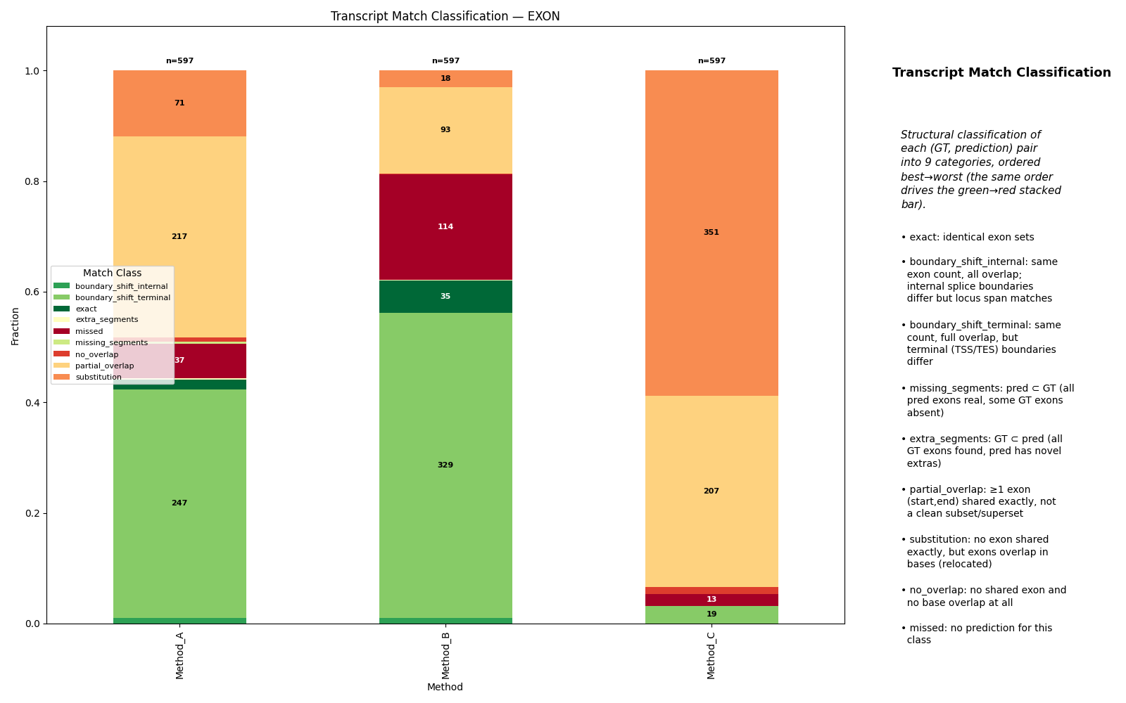
Transcript Classifications

Each (GT, prediction) pair is assigned one holistic structural class that summarises how the predicted transcript structure relates to the ground truth.

Transcript match classes

Class	Description
`exact`	Identical sets of `(start, end)` coding segments.
`boundary_shift_internal`	Same segment count and every predicted segment overlaps its positional GT counterpart; outer locus boundaries match, but one or more internal splice-site boundaries differ.
`boundary_shift_terminal`	Same segment count and full pairwise overlap, but one or both terminal (gene-locus start/end) boundaries differ.
`missing_segments`	Every predicted segment exists in GT (pred ⊂ GT) but some GT segments are absent — under-calling.
`extra_segments`	Every GT segment is found in the prediction (GT ⊂ pred) but the prediction adds novel segments — over-calling.
`partial_overlap`	At least one `(start, end)` pair is shared exactly but the sets are neither equal nor in a subset relationship. Captures collapsed or heavily altered structures.
`substitution`	No `(start, end)` pair is shared exactly, yet at least one predicted segment overlaps a GT segment in base coordinates — relocated or substituted exons.
`no_overlap`	No segment is shared exactly and no base-coordinate overlap exists between GT and prediction.
`missed`	The prediction contains no segments for this transcript (and GT does have segments).

If GT itself has no segments of this class the transcript is excluded from the match-class distribution rather than counted as missed — otherwise an empty reference would be reported as a prediction failure.

The two boundary-shift variants distinguish internal splice-site errors from changes that alter the reported gene-locus boundaries — a useful split because terminal boundary errors often reflect UTR ambiguity rather than splicing errors.

Representative examples

Exact match

GT exons: (100-180) (260-340) (420-500)
Pred exons: (100-180) (260-340) (420-500)
Class: exact

Splice-site shift (internal)

GT exons: (100-180) (260-340) (420-500)
Pred exons: (100-180) (255-345) (420-500)
Class: boundary_shift_internal — count unchanged, one internal boundary pair displaced.

Skipped middle exon

GT exons: (100-180) (260-340) (420-500)
Pred exons: (100-180) (420-500)
Class: missing_segments — transcript marked incomplete; Region Discovery may still give partial credit for retained exons.

Spurious extra exon

GT exons: (100-180) (260-340) (420-500)
Pred exons: (100-180) (260-340) (360-390) (420-500)
Class: extra_segments

Collapsed or heavily altered structure

GT exons: (100-180) (260-340) (420-500)
Pred exons: (100-210) (300-360) (420-500)
Class: partial_overlap — neither a clean subset/superset nor a pure boundary shift.

Missed transcript

GT exons: (100-180) (260-340) (420-500)
Pred exons: none
Class: missed — yields zero exon recall for that transcript.

Boundary Shift Distribution

For transcripts where GT and prediction have the same number of segments (i.e. transcripts classified as exact, boundary_shift_internal or boundary_shift_terminal), the benchmark records both a per-transcript summary and the individual per-boundary offsets:

boundary_shift_count — the number of individual boundary positions (segment starts and ends) that differ between GT and prediction.
boundary_shift_total — the cumulative base-pair offset summed across all shifted boundaries in that transcript.
boundary_shift_offsets — one record per shifted boundary, carrying its signed offset (pred − gt in array coordinates; positive means the edge moved to the right / array-3’) and a position tag of internal (an interior splice junction) or terminal (the transcript’s outer start/end, i.e. TSS/TES in array orientation).

These are only meaningful when segment counts match and every predicted segment overlaps its positional GT counterpart; if either fails all three are empty/zero and the transcript is excluded from the distribution plots. Note the conditioning: this view only describes transcripts whose chain topology is already correct, so it isolates junction-placement precision from the separate question of recovering the right exons. That makes it complementary to — not a duplicate of — the global boundary precision landscape, which pools every overlapping section pair regardless of topology.

Read eligibility before precision. Because the distribution is conditioned on topology-correct transcripts and only records boundaries that actually differ (exact, offset-0 junctions are dropped), a method that recovers correct topology for only a handful of easy transcripts can still show a tight, flattering offset distribution. The offset panels therefore say nothing about how many transcripts a method got right. To stop this being misread, the figure carries the denominator alongside the offsets: a leftmost transcript-match classification bar, and a per-method eligibility caption (the share of GT transcripts the panels are conditioned on, flagged ⚠ when below 25 %). Always read those together with the boxes — and consult the unconditional splice-site precision/recall and confusion plots for the full-recall picture.

Boundary shift distribution

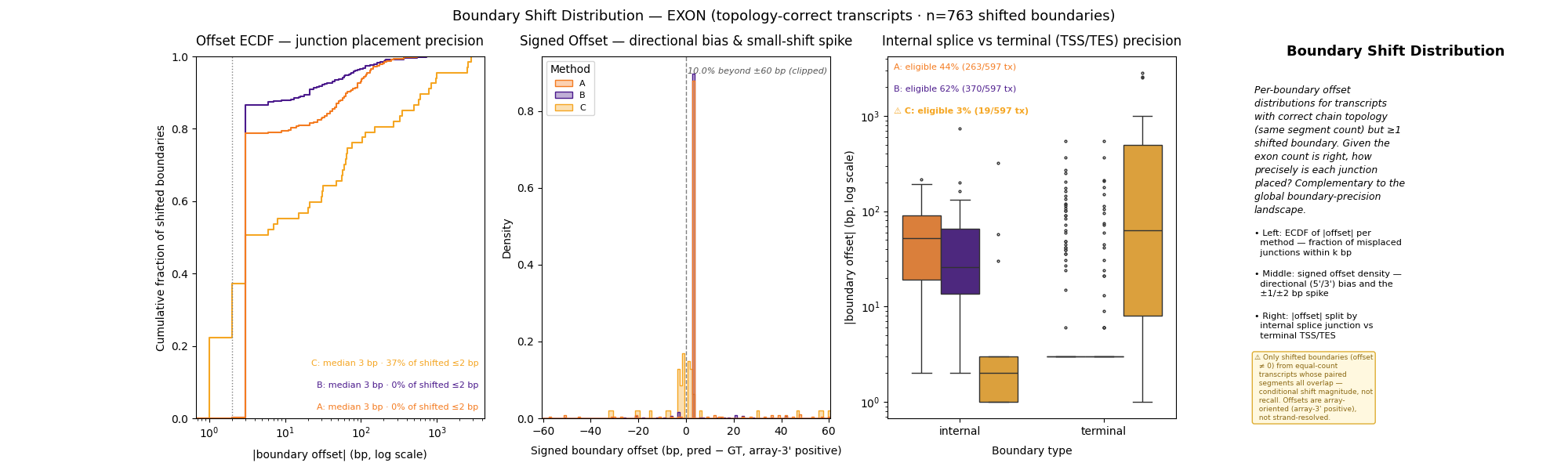
The four panels show:

Transcript match classes (leftmost) — the severity-graded classification stacked bar (see above), repeated here as the denominator for the offset panels. The eligible (topology-correct) classes exact / boundary_shift_internal / boundary_shift_terminal are what the remaining panels are conditioned on.
Offset ECDF (log x) — the cumulative distribution of |offset| per method, read as “fraction of shifted junctions within k bp”. The per-method median offset and the percentage of shifted boundaries within ±2 bp are annotated (exact junctions are excluded upstream, so this is not an overall junction-accuracy rate). Because it is a cumulative fraction, methods with very different numbers of shifted boundaries remain directly comparable. The dotted line marks the ±2 bp reference.
Signed Offset density — the signed offset over a robust window (the central ~98 % of the data; the clipped tail fraction is annotated). It exposes the heavy ±1/±2 bp spike typical of off-by-one splice-site errors and any directional bias: a histogram skewed right of zero indicates predicted edges systematically shifted toward array-3’.
Internal vs Terminal (log y) — |offset| split by boundary type. Internal splice junctions are, by biological convention, GT–AG-bounded and should be tight; terminal TSS/TES boundaries are inherently fuzzy. (The benchmark compares annotated junction positions, not nucleotide identity.) Separating them prevents transcript-end uncertainty from masking (or being mistaken for) genuine splice-site imprecision. This panel is overlaid with the per-method eligibility caption (topology-correct share, ⚠ below 25 %) so the boxes are always read against the size of the population they summarise.

Strand note. Offsets use array orientation (lower index = array-5’), not biological strand, so on the minus strand array-5’/3’ correspond to the biological 3’/5’ ends. A biological donor/acceptor decomposition is therefore deferred until minus-strand arrays are reverse-complemented upstream; the internal/terminal split above is strand-agnostic and unaffected.

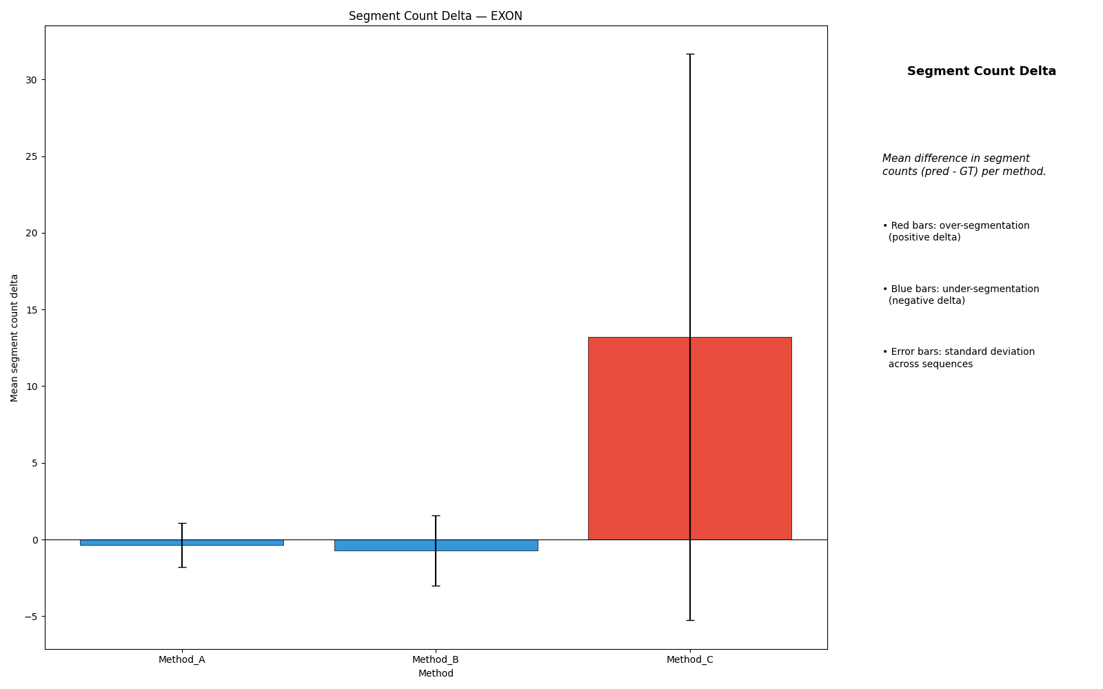
Segment Count Delta

segment_count_delta = pred_count − gt_count

This metric captures systematic over- or under-segmentation across the predicted transcriptome.

Positive values indicate over-segmentation (the predictor splits GT segments into more pieces than exist in the reference).
Negative values indicate under-segmentation (the predictor merges or omits GT segments).
Zero means the predicted segment count matches GT on average.

After aggregation the metric is summarised with mean and spread (rather than a single raw count) to expose both the direction and the consistency of the bias.

Segment count delta

Exon Recovery

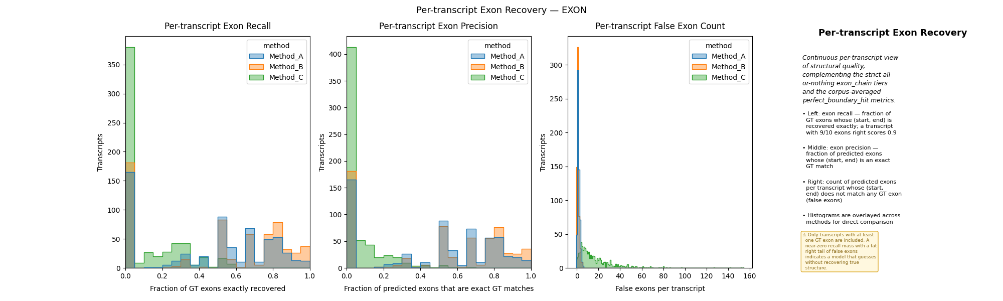
The strict chain score is deliberately all-or-nothing. The exon-recovery metrics add a distributional view that quantifies how far off a prediction is even when the strict score fails. Matching is still exact (start, end) identity — the gradation is in the fraction matched, not in any boundary tolerance.

Exon recovery

Exon recall per transcript

exon_recall_per_transcript is the fraction of GT exons that are recovered exactly in the prediction, computed per (GT, prediction) pair and then summarised across the corpus.

A value of 1.0 means every GT exon boundary was reproduced exactly. Lower values indicate how many GT exons are systematically missed, regardless of whether the overall chain score is a pass or fail.

Exon precision per transcript

exon_precision_per_transcript is the fraction of predicted exons whose (start, end) is an exact GT match, the symmetric precision partner to recall. It is 0.0 when the prediction has no exons in scope.

A value of 1.0 means every predicted exon is real. Lower values indicate that the predictor emits exons not present in the reference.

False exon count per transcript

false_exon_count_per_transcript is the number of predicted exons that have no exact counterpart in the GT set, computed per transcript pair. It is the absolute spurious-exon burden that the precision ratio hides (two false exons mean very different things in a 2-exon and a 40-exon transcript).

Higher values indicate that the predictor invents exon boundaries not present in the reference. Note that this count is independent of recall: a method can simultaneously recover all GT exons (high recall) while also adding spurious ones (high false-exon count).

Reading the metrics together

Exon recall	False count	Interpretation
High	Low	Mostly correct transcript recovery.
High	High	GT structure is covered but the predictor also invents extra exons.
Low	Low	Conservative under-calling — few false exons but many GT exons missed.
Low	High	Heavily incorrect predictions: both missing GT exons and spurious new ones.

Splice-Site Junctions

The chain and boundary-shift metrics above treat each intron junction as a single boundary pair. The splice-site metrics instead split every junction into its two halves — the donor (5′ splice site) and the acceptor (3′ splice site) — and score them independently. This isolates whether a predictor tends to place one end of a junction correctly while missing the other.

This block (splice_site_results) is only emitted when the label scheme defines all three of intron_label, splice_donor_label, and splice_acceptor_label. Without them the key is absent and the plots below are skipped.

Junction pairing

GT junctions are reconstructed by walking the segment chain in order: a valid junction is a donor segment, followed by zero or more intron segments, followed by an acceptor segment. Each such donor/acceptor pair becomes one scored junction. A donor that is never closed by an acceptor, or an acceptor with no preceding donor, is malformed — counted separately (see below) rather than scored.

A predicted donor or acceptor counts as a hit only when it matches the GT segment exactly — identical (start, end) span. This is the same exact-match philosophy as the strict chain score, applied to individual splice sites.

Donor/acceptor confusion

For every valid GT junction the benchmark records whether each half was recovered, yielding a 2×2 outcome:

Outcome	Donor	Acceptor
`both_correct`	hit	hit
`donor_only`	hit	miss
`acceptor_only`	miss	hit
`neither`	miss	miss

Splice-site junction confusion

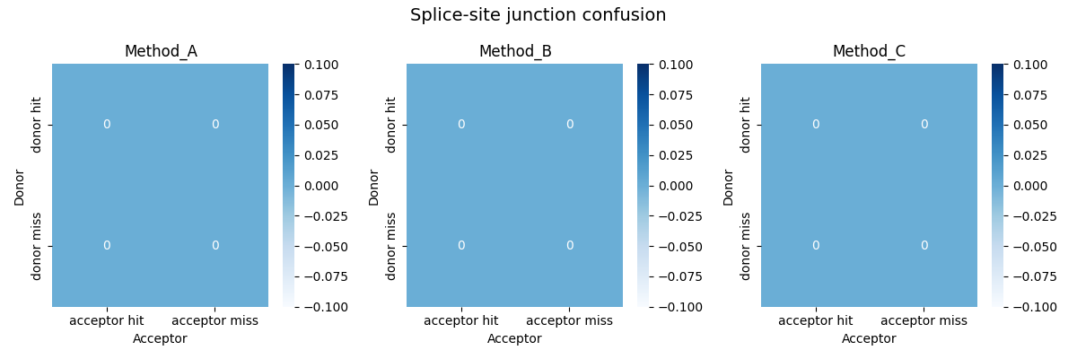
Mass concentrated in both_correct means whole junctions are reproduced; weight in donor_only or acceptor_only exposes a 5′/3′ asymmetry where one splice site is systematically harder to place than the other.

Precision and recall

The two halves are also scored as independent detection problems. Per GT junction a recovered donor is a true positive and a missed donor a false negative; any predicted donor that does not match the donor of a valid GT junction is a false positive (acceptors likewise). Aggregation sums these counts across the corpus and derives:

donor_precision, donor_recall
acceptor_precision, acceptor_recall

Splice-site precision & recall

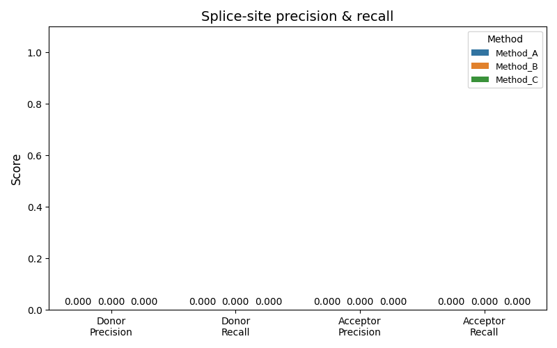
Precision penalises hallucinated splice sites; recall penalises missed ones. Contrasting donor against acceptor precision/recall surfaces the same 5′/3′ asymmetry as the confusion view, on a 0–1 scale that stays comparable across datasets with different junction counts.

Malformed junctions

gt_malformed_junctions and pred_malformed_junctions count donor/acceptor labels that never form a valid donor → intron* → acceptor pairing. GT malformed junctions are dropped from the pair list, so they contribute no donor/acceptor true positives or false negatives; both counts are reported as data-quality diagnostics and emit a warning when non-zero. A persistently high malformed count usually points to a label-scheme or post-processing problem rather than a biological splicing error.

Caveats

intron_chain requires intron labels or infer_introns=True when introns should be inferred from coding gaps.
Splice-site junction metrics require intron_label, splice_donor_label, and splice_acceptor_label to all be configured; otherwise no splice_site_results are produced.
Good Region Discovery scores do not guarantee good Structural Coherence. A model can recover many individual sections while still assembling the wrong transcript chain.
Exon-recovery metrics operate on exact coding-segment boundaries, not fuzzy overlaps.